
Estimation and Confidence Intervals#
In this chapter, we will investigate methods for learning about (also called estimating) a population characteristic (called parameter). The diagram below shows the assumptions we will build on:
We have a population of interest (for example, the annual salaries for all City of Chicago empolyees).
The interest is in a parameter (a numerical characteristic) of that population denoted by \(\theta\) (for example, median salary for all City of Chicago employees).
A sample of size \(n\) is drawn from the population using a specified sampling scheme (for example, a simple random sample).
From the data in the sample, a statistic \(\hat\theta\) is calculated (for example, the median of the salaries in the sample); this statistic is used as an estimate for the parameter of interest.

The data shown below was downloaded from the City of Chicago in June, 2023 and contains data for 24,365 employees. The file was processed to simplify our illustration here: some columns that are not needed were removed, and only rows having data on annual salaries were retained. Five random data points (rows in the data frame) are shown.
population_salary=pd.read_csv("../data/Salaries.csv")
population_salary.shape
(24365, 3)
population_salary.sample(5,replace=False)
| Job Titles | Department | Annual Salary | |
|---|---|---|---|
| 19070 | POLICE COMMUNICATIONS OPERATOR I | OFFICE OF EMERGENCY MANAGEMENT | 55932.0 |
| 15236 | SR RECOVERY TEAM PROGRAM MGR | DEPARTMENT OF PUBLIC HEALTH | 123864.0 |
| 3171 | POLICE OFFICER (ASSIGNED AS DETECTIVE) | DEPARTMENT OF POLICE | 109704.0 |
| 1462 | SERGEANT | DEPARTMENT OF POLICE | 125634.0 |
| 19585 | SUPERVISING POLICE COMMUNICATIONS OPERATOR | OFFICE OF EMERGENCY MANAGEMENT | 109872.0 |
The above data represents our population, and we assume we are interested in the median salary - this is the parameter of interest, and it is equal to $101,262 as shown by output of the cell code below:
theta=population_salary['Annual Salary'].median()
theta
101262.0
Suppose we would like to learn about this parameter not by collecting the data on the whole population, which can be expensive and/or impractical, but by obtaining a simple random sample of size, let’s say, \(n=100\). We simulate this process below twice.
np.random.seed(1234)

# a simple random sample of 100 observations (rows)
sample1_salary=population_salary.sample(100,replace=False)

# the median salary in the sample
theta_hat1=sample1_salary['Annual Salary'].median()
theta_hat1
98904.0
Recall that we introduced and discussed the role of np.random.seed in Section 10.3.
np.random.seed(4321)

# a simple random sample of 100 observations (rows)
sample2_salary=population_salary.sample(100,replace=False)

# the median salary in the sample
theta_hat2=sample2_salary['Annual Salary'].median()
theta_hat2
100644.0
As you can see above, different samples will lead to different estimated values - some closer and some further away from the true value. To understand the properties of our estimate (its accuracy, for example), we need to understand its sampling distribution - see Chapter 12 for a more in-depth discussion of distributions. The picture below shows a schematic that provides intuition on the sampling distribution:

The sampling distribution can be approximated by calculating the statistic of interest in repeated samples drawn using the same sampling scheme and with the same sample size.
Below, we construct an approximation for the sampling distribution of the sample median in simple random samples of size 100. We simulate 10,000 simple random samples and calculate their medians.
# the array where sample medians will be stored
sampling_distribution=np.array([])

# the number of samples we will generate
n_sample=10000

for i in range(n_sample):
    sampling_distribution=np.append(sampling_distribution,
                          population_salary.sample(100,replace=False)['Annual Salary'].median())
# histogram of the 10,000 sample medians
# this is an approximation of the sampling distribution
plt.hist(sampling_distribution,bins=np.arange(96000,108000,1000))
plt.title('10,000 simulated samples')
plt.xlabel("Sample medians");
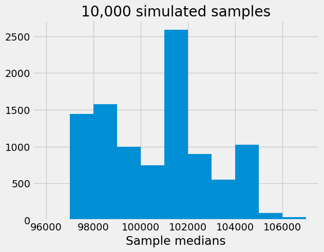
Note that properties of the estimator are reflected by its sampling distribution. From the above plot:
The true value ($101,262) seems to be close to the center of the histogram;
Most of the sample medians are within $3-4,000 of the population median.
It is clear that if we report only the estimator, we provide incomplete information on the population parameter. The second bullet point above suggests that we can report a range of plausible values that has a good chance of capturing the parameter. A plausible range of values for the population parameter is called a confidence interval (CI).