Categorical data
Categorical data#
Categorical variables represent the type of data that are labeled and divided into groups. Examples include race, gender, college major, political preference, coin tossing outcome (heads or tails), etc.
Testing for two-sample differences in categorical data can be done using the same procedures we introduced for numerical observations. The main difference is in the choice of test statistic and we illustrate it below with data from the 2022 General Social Survey.
gss=pd.read_csv("../../data/gss.csv")
gss
| Sex | Strong democrat | Not very strong democrat | Independent, close to democrat | Independent (neither, no response) | Independent, close to republican | Not very strong republican | Strong republican | Other party | |
|---|---|---|---|---|---|---|---|---|---|
| 0 | MALE | 198 | 197 | 169 | 366 | 256 | 206 | 222 | 76 |
| 1 | FEMALE | 320 | 264 | 181 | 409 | 162 | 174 | 225 | 39 |
The table above shows the number of subjects by gender and party identification (for example, there are 198 subjects who identify as “Male” and “Strong democrat”. The goal of the analysis is to investigate if there are differences in party identification between males and females. As you can see below, there are 1690 males and 1774 females in this dataset.
gss.drop(columns=["Sex"]).sum(axis=1)
0    1690
1    1774
dtype: int64
To test if males and females have the same party identification distributions, we need to set up the components of a hypothesis test:
Null hypothesis, \(H_0\) - the proportion of males and females in each party category in the US population are the same.
Alternative hypothesis, \(H_A\) - there is at least one category for which the proportions are different.
Test statistic - because we are interested in finding differences in proportions, it is natural to consider functions of these differences, such as total variation distance introduced below.
Total variation distance (TVD) is defined as the sum of absolute differences in proportions:
In the above formula, \(p_i\)’s are proportions of subjects in various categories (e.g. party identification) in one sample (e.g., males) while \(q_i\)’s are proportions in the second sample (e.g., females).
A function that calculates the total variation distance for two arrays of counts is implemented below.
def tvd(array1,array2):
    """ Total variation distance for proportions from two arrays of counts"""
    return sum(abs(array1/sum(array1)-array2/sum(array2)))/2

obs_TVD=tvd(gss.drop(columns=["Sex"]).iloc[0].values,
          gss.drop(columns=["Sex"]).iloc[1].values)

print(obs_TVD)
0.11148542724295041
For our data, TVD between males and females is equal to 0.11. Next, we will determine if this value is consistent with our null hypothesis.
Note that the data is in aggregated form. To implement the permutation procedure, we need to create first a dataframe that has 1690+1774=3464 rows, with each row corresponding to one participant in the study. The data frame will capture information on sex and party preference. A sample of 5 rows in the new data frame is displayed.
# arrays of the categories in the two variables
sex=gss.Sex.values
party=gss.drop(columns=["Sex"]).columns.values

# start with an empty dataframe
gss_full=pd.DataFrame()

# for each count in the `gss` data frame, add a corresponding number of rows
for i in sex:
    for j in party:
        nr_sub=gss[gss.Sex==i][[j]].values.item()
        df=pd.DataFrame([list([i,j])],index=range(nr_sub),columns=list(["Sex","Party"]))
        gss_full=pd.concat([gss_full,df])

gss_full.sample(5)
| Sex | Party | |
|---|---|---|
| 156 | FEMALE | Independent, close to democrat |
| 89 | FEMALE | Strong democrat |
| 135 | FEMALE | Not very strong democrat |
| 201 | MALE | Independent (neither, no response) |
| 178 | FEMALE | Independent, close to democrat |
Note that we can calculate the number of subjects in each group using groupby, and from this summary we can calculate TVD.
tmp=gss_full.groupby(["Sex","Party"]).size()
tmp
Sex     Party
FEMALE  Independent (neither, no response)    409
        Independent, close to democrat        181
        Independent, close to republican      162
        Not very strong democrat              264
        Not very strong republican            174
        Other party                            39
        Strong democrat                       320
        Strong republican                     225
MALE    Independent (neither, no response)    366
        Independent, close to democrat        169
        Independent, close to republican      256
        Not very strong democrat              197
        Not very strong republican            206
        Other party                            76
        Strong democrat                       198
        Strong republican                     222
dtype: int64
tvd(tmp.values[0:8],tmp.values[8:16])
0.11148542724295042
Above, we illustrated that our procedure for constructing the sampling frame (the raw dataset) is correct - we obtained the same test statistic from the complete data table as the one we obtained from the summary data.
We are ready now to simulate under the null hypothesis using permutations.
# the array where simulated TVDs will be stored
sim_tvd=np.array([])

# the number of simulations
nr_sim=1000

for i in np.arange(nr_sim):
    gss_full_copy=gss_full
    gss_full_copy['Party']=np.random.permutation(gss_full_copy['Party'])
    tmp=gss_full_copy.groupby(["Sex","Party"]).size()
    sim_tvd=np.append(sim_tvd,tvd(tmp.values[0:8],tmp.values[8:16]))
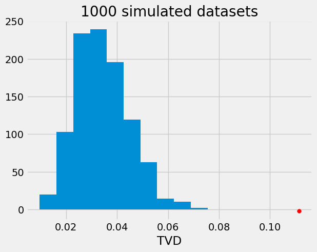
The simulation results are saved in an array, sim_tvd, of length 1000. We created 1000 shuffled datasets and for each we calculated the corresponding TVD value. The histogram below shows that there is strong evidence against the null hypothesis that men and women had the same distribution of political differences.
plt.hist(sim_tvd)
plt.scatter(obs_TVD, -2, color='red', s=30)
plt.title('1000 simulated datasets')
plt.xlabel("TVD");