Grouping Data#

In addition to merging multiple DataFrames, we can perform operations within a single DataFrame.

The groupby function allows us to split the DataFrame into groups. We can extract the grouped data directly into a new DataFrame or apply a specified function before combining the results into a DataFrame. The most important input to this function is what we are grouping by, usually a column name. The general format of the groupby operation is given by:

df.groupby(by='group_name'),

where ‘group_name’ specifies the column name of which to group by unique entries in the column.

We’ll redefine the merged right menu to use in our investigation with grouping below.

nutritional_info = pd.DataFrame({
    'Item': ['Big Mac', 'Medium French Fries', 'Cheeseburger', 'McChicken', 'Hot Fudge Sundae', 'Sausage Burrito', 'Baked Apple Pie'],
    'Calories': [530, 340, 290, 360, 330, 300, 250],
    'Protein': [24, 4, 15, 14, 8, 12, 2],
})

menu = pd.DataFrame({
    'Item': ['Big Mac', 'Cheeseburger', 'McChicken', 'Hot Fudge Sundae', 'Egg McMuffin', 'Medium French Fries', 'Sausage Burrito'],
    'Price': [5.47, 1.81, 2.01, 2.68, 4.43, 2.77, 2.10],
    'Category': ['Lunch/Dinner', 'Lunch/Dinner', 'Lunch/Dinner', 'Dessert', 'Breakfast', 'Lunch/Dinner', 'Breakfast'],
})

full_menu = pd.merge(nutritional_info, menu, how='right')

full_menu

	Item	Calories	Protein	Price	Category
0	Big Mac	530.0	24.0	5.47	Lunch/Dinner
1	Cheeseburger	290.0	15.0	1.81	Lunch/Dinner
2	McChicken	360.0	14.0	2.01	Lunch/Dinner
3	Hot Fudge Sundae	330.0	8.0	2.68	Dessert
4	Egg McMuffin	NaN	NaN	4.43	Breakfast
5	Medium French Fries	340.0	4.0	2.77	Lunch/Dinner
6	Sausage Burrito	300.0	12.0	2.10	Breakfast

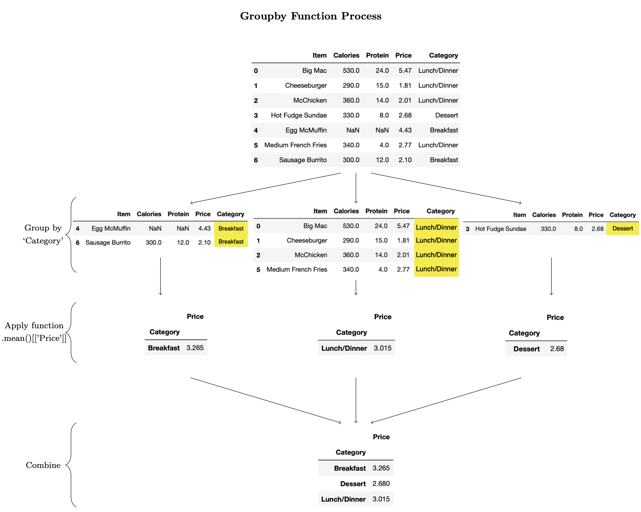
We can use full_menu above and group the items by “Category”. The groupby function by itself splits the data. If we want to form a new DataFrame or add a computation, this must be specified.

Here we create a new DataFrame using the get_group method. This creates a new DataFrame with entries from the specified group; in this case only items from the category “Breakfast” are included in the DataFrame.

category_groups = full_menu.groupby('Category') 

category_groups.get_group('Breakfast')

	Item	Calories	Protein	Price	Category
4	Egg McMuffin	NaN	NaN	4.43	Breakfast
6	Sausage Burrito	300.0	12.0	2.10	Breakfast

Applying Functions within Groupby#

In addition to viewing or sorting the data, the groupby operation is useful in applying functions to groups of a DataFrame.

Perhaps we want to know the average price, grouped by the category of each item. We use the line below, which first groups the data by “Category” and then takes the mean across the “Price” column within each group.

(The double brackets around 'Price' are needed to ensure we get a DataFrame as output. See: DataFrames: Selection by label.)

full_menu.groupby('Category')[['Price']].mean()

	Price
Category
Breakfast	3.265
Dessert	2.680
Lunch/Dinner	3.015

The groupby operation allows us to split the DataFrame into groups, apply a specified function, and combine the results into a DataFrame. The behind the scenes process of this code is outlined below.

There are many different functions we can apply to our groups. Common functions include: count, min, max, sum, mean, std, var. (For more information, consult the pandas documentation of groupby.)

We demonstrate a few of these functions below.

For example, it might be useful to count how many items on the full_menu fall into each “Category”: “Breakfast”, “Lunch/Dinner”, and “Dessert”. We can do so by first grouping the DataFrame by “Category” and then counting how many “Items” are in each group.

full_menu.groupby('Category')[['Item']].count()

	Item
Category
Breakfast	2
Dessert	1
Lunch/Dinner	4

Or, perhaps we want to sum the menu prices by “Category”. We first group by “Category” and then add up all prices within each group:

full_menu.groupby('Category')[['Price']].sum()

	Price
Category
Breakfast	6.53
Dessert	2.68
Lunch/Dinner	12.06

Grouping on a Larger Dataset#

To see the full potential of grouping, we’ll consider a larger DataFrame. We consider the Data Science Jobs and Salaries dataset which contains information on:

Data Science job titles
experience level: Entry-level (EN), Mid-level (MI), Senior-level (SE), Executive-level (EX)
remote vs full time ratio
2020 salary or 2021 expected salary (2021e)
employment type: PT (part time), FT (full time), CT (contract), FL (Freelance)

(For a more complete view of the data, note that they were taken from Saurabh Shahane at Kaggle, which gathered information from ai-jobs.net.)

salary_data = pd.read_csv("../../data/Data_Science_Jobs_Salaries.csv")
salary_data.head(5)

	work_year	experience_level	employment_type	job_title	salary	salary_currency	salary_in_usd	employee_residence	remote_ratio	company_location	company_size
0	2021e	EN	FT	Data Science Consultant	54000	EUR	64369	DE	50	DE	L
1	2020	SE	FT	Data Scientist	60000	EUR	68428	GR	100	US	L
2	2021e	EX	FT	Head of Data Science	85000	USD	85000	RU	0	RU	M
3	2021e	EX	FT	Head of Data	230000	USD	230000	RU	50	RU	L
4	2021e	EN	FT	Machine Learning Engineer	125000	USD	125000	US	100	US	S

This is only the first few and the last few rows; this DataFrame contains a lot of information! We can extract or sort the information we want by grouping the data in a convenient way. The groupby method in pandas will help us do exactly that!

For example, we can group the salary_data by the experience level of the employees. Recall we may do this by first splitting the data into experience_level groups and then extracting the group of employees with experience_level equal to EN, or entry-level experience. The resulting DataFrame contains only entries from the specified group: entry-level experience employees.

experience_level_groups = salary_data.groupby('experience_level')

experience_level_groups.get_group('EN').head(5)

	work_year	experience_level	employment_type	job_title	salary	salary_currency	salary_in_usd	employee_residence	remote_ratio	company_location	company_size
0	2021e	EN	FT	Data Science Consultant	54000	EUR	64369	DE	50	DE	L
4	2021e	EN	FT	Machine Learning Engineer	125000	USD	125000	US	100	US	S
11	2021e	EN	FT	Data Scientist	13400	USD	13400	UA	100	UA	L
17	2021e	EN	FT	Data Analyst	90000	USD	90000	US	100	US	S
18	2021e	EN	FT	Data Analyst	60000	USD	60000	US	100	US	S

We can group by more than one category as well. Below we group first by employment_type and within each employment_type group we group by experience_level. The first method then return the first row, if it exists, of each group.

two_groups = salary_data.groupby(['employment_type','experience_level']) 

two_groups.first()

		work_year	job_title	salary	salary_currency	salary_in_usd	employee_residence	remote_ratio	company_location	company_size
employment_type	experience_level
CT	EN	2020	Business Data Analyst	100000	USD	100000	US	100	US	L
	EX	2021e	Principal Data Scientist	416000	USD	416000	US	100	US	S
	MI	2021e	ML Engineer	270000	USD	270000	US	100	US	L
	SE	2021e	Staff Data Scientist	105000	USD	105000	US	100	US	M
FL	MI	2021e	Data Engineer	20000	USD	20000	IT	0	US	L
FL	SE	2020	Computer Vision Engineer	60000	USD	60000	RU	100	US	S
FT	EN	2021e	Data Science Consultant	54000	EUR	64369	DE	50	DE	L
	EX	2021e	Head of Data Science	85000	USD	85000	RU	0	RU	M
	MI	2020	Research Scientist	450000	USD	450000	US	0	US	M
	SE	2020	Data Scientist	60000	EUR	68428	GR	100	US	L
PT	EN	2021e	AI Scientist	12000	USD	12000	PK	100	US	M
PT	MI	2021e	3D Computer Vision Researcher	400000	INR	5423	IN	50	IN	M

Having grouped the data into single or multiple categories, we’ll now apply functions to these categories!

Perhaps we want to know the average salary grouped by experience level. We use the line below, which groups the data by experience_level and takes the mean across the salary_in_usd column within each group.

salary_data.groupby('experience_level').salary_in_usd.mean() 

experience_level
EN     59753.462963
EX    226288.000000
MI     85738.135922
SE    128841.298701
Name: salary_in_usd, dtype: float64

We can also count how many people work (or get salaries) at each size company: small, medium, large.

First we group different company sizes and count all employees who receive a salary.

(Recall that the double brackets on 'salary' ensure our result is a DataFrame and not a series. The output above, for average salary by experience level, was a simple series – see if you can write this as a DataFrame!)

salary_data.groupby('company_size').count()[['salary']]

	salary
company_size
L	132
M	55
S	58

Additionally, the groupby method can be used to split the data into multiple groups, apply a function, and then reform it into a DataFrame.

Similar to the above example, we first group by multiple columns, subdividing into experience_level and then further by company_size:

experience_and_compsize = salary_data.groupby(['experience_level', 'company_size'])

experience_and_compsize.first()

		work_year	employment_type	job_title	salary	salary_currency	salary_in_usd	employee_residence	remote_ratio	company_location
experience_level	company_size
EN	L	2021e	FT	Data Science Consultant	54000	EUR	64369	DE	50	DE
	M	2021e	PT	AI Scientist	12000	USD	12000	PK	100	US
	S	2021e	FT	Machine Learning Engineer	125000	USD	125000	US	100	US
EX	L	2021e	FT	Head of Data	230000	USD	230000	RU	50	RU
	M	2021e	FT	Head of Data Science	85000	USD	85000	RU	0	RU
	S	2021e	FT	Data Science Consultant	59000	EUR	70329	FR	100	ES
MI	L	2020	FT	Data Analyst	41000	EUR	46759	FR	50	FR
	M	2020	FT	Research Scientist	450000	USD	450000	US	0	US
	S	2021e	FT	Machine Learning Engineer	40000	EUR	47681	ES	100	ES
SE	L	2020	FT	Data Scientist	60000	EUR	68428	GR	100	US
	M	2021e	FT	Data Analytics Manager	120000	USD	120000	US	100	US
	S	2021e	FT	Data Analyst	80000	USD	80000	BG	100	US

If we want to compute the average salary within each experience level and dependent on company size we can use our multi-grouped DataFrame and aggregate the average salary:

experience_and_compsize['salary_in_usd'].mean()

experience_level  company_size
EN                L                75148.000000
                  M                41063.923077
                  S                57502.000000
EX                L               239729.875000
                  M                85000.000000
                  S               243164.500000
MI                L                96285.451613
                  M                83982.800000
                  S                47610.000000
SE                L               134465.604651
                  M               122572.125000
                  S               120978.055556
Name: salary_in_usd, dtype: float64

From this we can see that the average salary for an entry level employee at a large company is $75,148.

To turn this Series into a DataFrame, we use the unstack method, which pivots the inner-most group, company_size, and rearranges as columns.

experience_and_compsize['salary_in_usd'].mean().unstack()

company_size	L	M	S
experience_level
EN	75148.000000	41063.923077	57502.000000
EX	239729.875000	85000.000000	243164.500000
MI	96285.451613	83982.800000	47610.000000
SE	134465.604651	122572.125000	120978.055556

This idea of splitting a DataFrame into multiple groups and computing multi-dimensional aggregations of values is such an important feature that it has its own function in pandas! It is called a pivot_table. In the next section, we introduce how to manipulate DataFrames using the pivot_table method.

Introduction to Data Science I & II

Grouping Data

Contents

Grouping Data#

Applying Functions within Groupby#

Grouping on a Larger Dataset#