The percentile bootstrap confidence intervals

We introduce here a different version of the bootstrap confidence interval. Although it is very popular, it is based on more assumptions. Here we assume that the sampling distribution for \(\hat\theta\) is known and that it is symmetric around \(\theta\); see below.

Then, \(U_1-\theta=\theta-L_1=W\) (reflecting the width of this distribution). From the picture above, with probability 0.90:

\[|\hat\theta-\theta|\leq W\]

leading to

\[\hat\theta-W\leq \theta\leq \hat\theta+W\]

We call \([ \hat\theta-W, \hat\theta+W]\) a 90% confidence interval. This can be approximated by \([L_1,U_1]\) and we call this a 90% confidence interval.

It leads to the following procedure for obtaining a confidence interval:

• use bootstrap to obtain an estimate of the sampling distribution of \(\hat\theta\).

• from the bootstrap distribution calculate the empirical percentiles \(L_1^b\) and \(U_1^b\)

• \([L_1^b,U_1^b]\) is called a percentile bootstrap CI.

We will illustrate this with the salary data - let’s assume that the interest now is on the population mean (the average salary of the City of Chicago employees).

# the parameter of interest
theta=population_salary['Annual Salary'].mean()

np.random.seed(3322)

# this is a SRS of size n=80
sample_salary=population_salary.sample(80,replace=False)

#the average salary in the sample
theta_hat=sample_salary['Annual Salary'].mean()

[theta,theta_hat]

[100382.64415185717, 97993.725]

Above, we calculate the average salary in the population (\(\$100,382.6\)) and in a simple random sample of size 80 (\(\$97,993.7\)). Below, we define a function that is very similar to the one introduced in the previous section, that generates bootstrap means needed for the approximation of the sampling distribution.

def bootstrap_mean(original_sample, label, replications):
    """Simulate sample means:
    original_sample: df containing the original sample data
    label: label of column containing the variable
    replications: number of bootstrap samples
    Returns array of bootstrap sample means
    """
    means = np.array([])
    for i in np.arange(replications):
        bootstrap_sample = original_sample.sample(len(original_sample),replace=True)
        resampled_mean = bootstrap_sample['Annual Salary'].mean()
        means = np.append(means, resampled_mean)
        
    return means

bstrap_means = bootstrap_mean(sample_salary, 'Annual.Salary', 1000)

plt.hist(bstrap_means)
plt.scatter(theta_hat, -10, color='purple', s=40)
plt.scatter(theta, -10, color='red', s=40)
plt.xticks(ticks=[92000,95000,98000,101000,104000], labels=["92K","95K","98K","101K","104K"])
plt.xlabel("bootstrap medians");

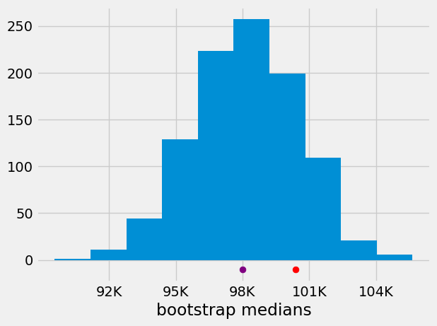
The above histogram is our approximation for the sampling distribution of \(\hat\theta\). The purple dot is the location of the average salary in our sample, and the red dot is the location of the average salary in the population.

left = np.percentile(bstrap_means, 2.5)
right = np.percentile(bstrap_means,97.5)

# a 95% CI
print([left,right])

[93339.230625, 102538.108125]

The 95% confidence interval for the average salary in the city of Chicago is [933339.2,102538.1].