
Arrays#
Evelyn Campbell, Ph.D.
An array is a data structure that consists of a collection of elements organized into a grid-like shape. In Python, arrays can be one-dimensional, akin to a list, or multidimensional (2D, 3D, etc.). However, unlike a list, an array consists of elements that are all of the same data type. This makes arrays convenient for storage and manipulation of data elements. Arrays are offered through the numpy library, and are often used in conjunction with other Python libraries, such as pandas, scipy, and scikit-learn (linked below). We will explore arrays in this section, along with commonly used functions used with arrays.
Constructing arrays#
To make an array, we first need to import numpy. This makes the methods in the numpy library available to us in our current Python session. Two useful functions in numpy are array() which creates numpy arrays from other data types and arange() which creates arrays containing regularly spaced floating-point numbers. After import numpy as np we can use these methods by prepending np. to their names: np.array() and np.arange()
import numpy as np

my_list = [30, 50, 70, 90]
my_array = np.array(my_list)
my_array
array([30, 50, 70, 90])
We see here that np.array() can make an array. The np.arange() function can also create arrays. arange() generates arrays of (floating-point) numbers with uniform spacing. When invoked with one argument, arange() generates a list of numbers starting with 1:
my_array1 = np.arange(10)
my_array1
array([0, 1, 2, 3, 4, 5, 6, 7, 8, 9])
When used (“called”) with two arguments, np.arange(start, stop) begins at start and ends before stop:
my_array2 = np.arange(4, 8)
my_array2
array([4, 5, 6, 7])
And with three arguments, np.arange(start, stop, step) begins at start, ends before stop, and has an interval step between adjacent elements:
my_array3 = np.arange(100,200,10)
my_array3
array([100, 110, 120, 130, 140, 150, 160, 170, 180, 190])
So far, these have been one-dimensional arrays. Arrays have an attribute .shape that is a tuple that counts the number of elements in each dimension:
print(my_array1.shape, my_array2.shape, my_array3.shape)
(10,) (4,) (10,)
Each of these shapes has only one element; this tells us these are 1d numpy arrays.
Mathematical operations with arrays#
Arrays also allow for convenient elementwise calculations. For example, we can easily multiply our two arrays to obtain a new array of values.
my_array4 = my_array1 * my_array3
print(my_array1)
print(my_array3)
print(my_array4)
[0 1 2 3 4 5 6 7 8 9]
[100 110 120 130 140 150 160 170 180 190]
[   0  110  240  390  560  750  960 1190 1440 1710]
The resulting array consists of the products of element-by-element multiplication of the first two arrays. Keep in mind that when performing calculations with multiple arrays, the dimensions of the arrays must be compatible.
Performing elementwise operations on arrays of different shapes is called broadcasting, and a discussion on array shape compatibility in mathematical operations can be found in the referenced documentation on Array broadcasting in numpy below.
More simply, we can also perform a desired calculation on all elements of an array using scalar values:
my_array3 / 20 + 7
array([12. , 12.5, 13. , 13.5, 14. , 14.5, 15. , 15.5, 16. , 16.5])
Reshaping and combining arrays#
Arrays can also be reshaped and combined. We can use the np.reshape() function to change the first two arrays from a 1-dimensional 1x4 array to a 2-dimensional 2x2 array.
print(my_array)
print(my_array2)
[30 50 70 90]
[4 5 6 7]
reshape1 = np.reshape(my_array, (2,2))
reshape2 = np.reshape(my_array2, (2,2))
reshape1
array([[30, 50],
       [70, 90]])
reshape2
array([[4, 5],
       [6, 7]])
When combining arrays that have the same shape, we can use the np.row_stack() and np.column_stack() functions to concatenate the rows and columns of multiple arrays, respectively.
combined_col = np.column_stack((reshape1, reshape2))
combined_col
array([[30, 50,  4,  5],
       [70, 90,  6,  7]])
combined_row = np.row_stack((reshape1, reshape2))
combined_row
/tmp/ipykernel_191/2819659571.py:1: DeprecationWarning: `row_stack` alias is deprecated. Use `np.vstack` directly.
  combined_row = np.row_stack((reshape1, reshape2))
array([[30, 50],
       [70, 90],
       [ 4,  5],
       [ 6,  7]])
Array functions#
Construction and reshaping of arrays is an important consideration if you wish to perform aggregate functions on them. Some useful aggregate functions that can be performed on arrays include np.min(), np.max(), np.sum(), and np.average(). These functions can be applied to the entire array or across rows and columns.
print(reshape1)
[[30 50]
 [70 90]]
np.min(reshape1)
np.int64(30)
To apply these functions across columns of the array, use an axis=0 argument. To apply them across rows, use an axis=1 argument. The returned array will be the same length as the number of columns or rows.
np.sum(reshape1, axis=0)
array([100, 140])
np.average(reshape1, axis=1)
array([40., 80.])
We can retrieve individual elements of arrays with square brackets containing numbers for the indexes. Since combined_col is a 2d-array, we need two indexes. The conventional order is rows then columns.
print(reshape1)
[[30 50]
 [70 90]]
reshape1[0,1] # row 0, column 1
np.int64(50)
reshape1[1,1] # row 1, column 1
np.int64(90)
Remember that because of 0-based indexing; the element in the first row and first column is [0,0] and the element in the second row and second column is [1,1].
And subsets of the array can be retrieved by using slices for the indexes. Slices are of the form start:stop. If either start or stop is omitted, the slices go as far as possible (to the beginning or the ending of the array on that axis.
combined_col
array([[30, 50,  4,  5],
       [70, 90,  6,  7]])
combined_col[1, 1:3]
array([90, 6])
If we omit both start and stop, : is a symbol for an index that is shorthand for “all the elements”:
combined_col[:, 1:3] # This gives columns 1 and 2 for all the rows.
array([[50,  4],
       [90,  6]])
And slicing has one more trick: you can give slices three numbers by adding a second colon. The third number specifies a “step”, causing the slice to take non-adjacent cells:
my_array1
array([0, 1, 2, 3, 4, 5, 6, 7, 8, 9])
my_array1[2::] # The list from element 2 to the end
array([2, 3, 4, 5, 6, 7, 8, 9])
my_array1[2::2] # starting at 2, skipping every other element/Numpy
array([2, 4, 6, 8])
Like with lists, we can use numbers or slices like this if we want subsets of the arrays. Unlike lists, we can ask for two-dimensional slices by putting two slices inside the square brackets.
A number of other aggregate functions can be applied to transform elements within an array. These include np.sqrt(), np.square(), np.power(), np.log(), and many others.
np.power(reshape2, 3)
array([[ 64, 125],
       [216, 343]])
Indexing and Slicing#
1D arrays can be indexed similarly to how lists are indexed, as mentioned in the section 4.1.
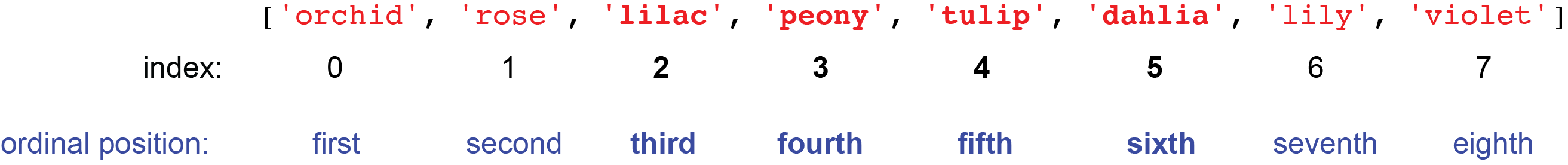
To begin in demonstrating this, let’s make a new array of string elements called flowers:
flowers = np.array(['orchid', 'rose', 'lilac', 'peony', 'tulip', 'dahlia', 'lily', 'violet'])
flowers
array(['orchid', 'rose', 'lilac', 'peony', 'tulip', 'dahlia', 'lily',
       'violet'], dtype='<U6')
As seen with lists, arrays utilize zero-indexing, meaning that the first element of an array has an index of 0. If we wanted to select the third to the sixth (inclusive) element in flowers, we need recognize that this corresponds to indexes 2 and 5, respectively.
A single colon (:) can be used to slice a range of elements in an array. The format for simple slicing an array is as follows:
array[start:end]
If used between the indices j and k, slicing the elements of an array will return all elements between j and k, excluding k.
In this case, we use 2:6 to slice from the third to the sixth element because we want to include the sixth element (which is located at index 5):
flowers[2:6]
array(['lilac', 'peony', 'tulip', 'dahlia'], dtype='<U6')
Arrays can also be sliced in intervals. Slicing in intervals takes on the following format:
array[start:end:step]
The step dictates the spacing between values. If we wanted to slice flowers starting at the second element to the sixth element (inclusive) in steps of two, we would use the following code:
flowers[1:6:2]
array(['rose', 'peony', 'dahlia'], dtype='<U6')
Slices can be made without explicitly indicating the start of end or the slice. In these cases, Python will start slicing with the first element if the beginning is not indicated and will stop at the last element if the end is not indicated:
flowers[1::2] # Starts at the second element and selects every other element to the end of the array
array(['rose', 'peony', 'dahlia', 'violet'], dtype='<U6')
flowers[:4] # Selects every element between the first and forth (inclusive) element
array(['orchid', 'rose', 'lilac', 'peony'], dtype='<U6')
When arrays become very long, it may be useful to use negative-indexing. Negative indexing assigns indices of elements starting from the last element. The very last element of an array has an index of -1, the penultimate, -2, and so on. If we want the fourth-from-last element of flowers, we could use the following:
flowers[-4]
np.str_('tulip')
Negative indexing can be combined with slicing to return elements of an array in a reverse order. For example, we can list all the flowers from lily to lilac in reverse order using the following:
flowers[6:1:-2]
array(['lily', 'tulip', 'lilac'], dtype='<U6')
Here, it’s okay that the starting index is greater than the ending index because we indicated the step to go from back to front.
Nested arrays#
When working with a multidimensional array, the same rules apply, but we have to keep in mind that the arrays within the a 2D array themselves have indices. Let’s construct two more arrays called fruits and pantone and make a combined array with flowers.
fruits = np.array(['strawberry', 'banana', 'blueberry', 'pineapple', 'cherry', 'papaya', 'lychee', 'mango'])
pantone = np.array(['emerald', 'polignac', 'saffron', 'fuchsia rose', 'marsala', 'ultra violet', 'mustard', 'lapis blue'])
combined = np.row_stack((flowers, fruits, pantone))
combined
/tmp/ipykernel_191/3411174661.py:3: DeprecationWarning: `row_stack` alias is deprecated. Use `np.vstack` directly.
  combined = np.row_stack((flowers, fruits, pantone))
array([['orchid', 'rose', 'lilac', 'peony', 'tulip', 'dahlia', 'lily',
        'violet'],
       ['strawberry', 'banana', 'blueberry', 'pineapple', 'cherry',
        'papaya', 'lychee', 'mango'],
       ['emerald', 'polignac', 'saffron', 'fuchsia rose', 'marsala',
        'ultra violet', 'mustard', 'lapis blue']], dtype='<U12')
We can assess the final dimensions of combined using the shape method. The shape method returns a tuple indicating the rows and columns:
combined.shape
(3, 8)
Now, we are working with an array of arrays that is 3 rows by 8 columns. As such, we have to be able to determine the index of each array to be able to even access the individual elements within them. For instance, if we wanted to identify the 3rd color within pantone, we first have to be able to index the array with colors:
combined[2]
array(['emerald', 'polignac', 'saffron', 'fuchsia rose', 'marsala',
       'ultra violet', 'mustard', 'lapis blue'], dtype='<U12')
Once we can get that array, getting the 3rd element would be as easy as identifying the index within pantone:
combined[2][2]
np.str_('saffron')
To this point, all of these slicing mechanisms are interchangeable between lists and arrays. However, if we wanted to take a particular index in all arrays of combined, the following would work for an array of arrays, but not a list of lists:
combined[:,2]
array(['lilac', 'blueberry', 'saffron'], dtype='<U12')
Notice that this gives a different result than the following code:
combined[:][2]
array(['emerald', 'polignac', 'saffron', 'fuchsia rose', 'marsala',
       'ultra violet', 'mustard', 'lapis blue'], dtype='<U12')
In slicing, a comma separates rows from columns. Hence, combined[:,2] is saying “from all rows of combined, take the column at index 2, while combined[:][2] is saying “from all elements in combined take the element at index 2.” This syntax, while subtle, greatly affects the granularity of slicing.
Ranges can also be used to slice specific subsets of columns and rows, as shown below:
combined[0:2,2:6]
array([['lilac', 'peony', 'tulip', 'dahlia'],
       ['blueberry', 'pineapple', 'cherry', 'papaya']], dtype='<U12')
We see that the above code returned the elements from index 2 to 5 (inclusive) from the flowers and fruits arrays within combined. The flowers and fruits arrays were returned because they are the elements at 0 and 1 index, respectively, within combined.
Using 2-D arrays to store and organize numerical data types can also be very useful. Below, we create a new array of array consisting of a collection of even numbers, numbers divisible by five, and numbers divisible by ten:
evens = np.arange(2.0, 11.0, 2)
fives = np.arange(5, 26, 5)
tens = np.arange(10, 51, 10)

num_comb = np.column_stack((evens, fives, tens))
num_comb
array([[ 2.,  5., 10.],
       [ 4., 10., 20.],
       [ 6., 15., 30.],
       [ 8., 20., 40.],
       [10., 25., 50.]])
We can use slicing to perform operations on specific subsets of num_comb:
num_comb[:][-1] + num_comb[3].sum()**2
array([4634., 4649., 4674.])
Furthermore, these slices can be used as input to functions:
np.power(num_comb[:,0], 2)
array([ 4., 16., 36., 64., 100.])
When working with multidimensional arrays, being able to subset portions and do calculations via functions or operations can be an easy way to analyze data, particularly, if the array is organized in a meaningful way. From this, new arrays can be created and appended to existing arrays to update or complete a dataset:
squared = np.power(num_comb[:,0], 2)

num_comb = np.column_stack((num_comb, squared))
num_comb
array([[  2.,   5.,  10.,   4.],
       [  4.,  10.,  20.,  16.],
       [  6.,  15.,  30.,  36.],
       [  8.,  20.,  40.,  64.],
       [ 10.,  25.,  50., 100.]])
Arrays are a powerful data type that make for easy and seamless data storage and analysis. The rules around slicing for arrays can be a bit tricky. It’s important to practice to get used indexing and to understand how to access arrays within arrays vs elements of said arrays.