
9.4. The birthday problem: relaxed assumptions#
There are two assumptions we used in the last few sections while investigating the birthday problem - equally likely birthdates and ignoring February 29 as a possible birth date. While relaxing these can complicate the mathematical calculation, the simulations can be easily modified to account for more complicated scenarios.
We use below a dataset from FiveThirtyEight that contains the number of daily births in US between 2000 and 2014 to estimate the odds of each day of the year to be a birthday:
Note that in the following dataset, the variable for day of week is coded 1 for Monday and 7 for Sunday. Also note that there are four leap years in this dataset - finding the correct probability for being born in a leap year is beyond the scope of this section.
birth_data = pd.read_csv("../../data/US_births_2000-2014_SSA.csv")
birth_data
| year | month | date_of_month | day_of_week | births | |
|---|---|---|---|---|---|
| 0 | 2000 | 1 | 1 | 6 | 9083 |
| 1 | 2000 | 1 | 2 | 7 | 8006 |
| 2 | 2000 | 1 | 3 | 1 | 11363 |
| 3 | 2000 | 1 | 4 | 2 | 13032 |
| 4 | 2000 | 1 | 5 | 3 | 12558 |
| ... | ... | ... | ... | ... | ... |
| 5474 | 2014 | 12 | 27 | 6 | 8656 |
| 5475 | 2014 | 12 | 28 | 7 | 7724 |
| 5476 | 2014 | 12 | 29 | 1 | 12811 |
| 5477 | 2014 | 12 | 30 | 2 | 13634 |
| 5478 | 2014 | 12 | 31 | 3 | 11990 |
5479 rows × 5 columns
This is an interesting dataset and we encourage you to use it to answer questions like: what is the least frequent day of the week for giving birth?
The pandas library has commands that allow you to group rows by unique values in a column. We introduced it in Chapter 7.
counts_df=birth_data.groupby(['month','date_of_month']).sum()[['births']]
counts_df.head(5)
| births | ||
|---|---|---|
| month | date_of_month | |
| 1 | 1 | 116030 |
| 2 | 144083 | |
| 3 | 170115 | |
| 4 | 171663 | |
| 5 | 166682 |
We see that there were 116,030 births on January 1st, 144,083 (much larger! why?) on January 2nd etc. A histogram of the counts in the above data frame:
plt.hist(counts_df.births,bins = np.arange(116000, 195000, 2000))
plt.xticks(ticks=[130000,150000,170000,190000], labels=["130K","150K","170K","190K"])
plt.xlabel("Number of births")
plt.ylabel("Frequency")
plt.show()
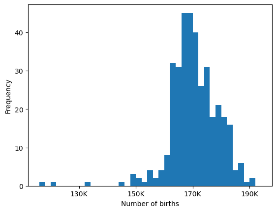
Note that some days of the year are outliers in number of births. Can you guess which?
We will use these counts to estimate the probability that a given date is a birthday for a random US subject.
bday_probs=counts_df.births/sum(counts_df.births)
These probabilities are added to the simulation when using the random.choice function. Look at the function below and compare it to the birthday_sim function introduced in Section 10.2.
# adding February 29 - the number of possible birthdays is now 366
birthdays2=np.arange(1,367,1)

def birthday_sim2(n,nrep,pr):
    '''Estimate birthday matching probabilities using nrep simulations.
       The 366 possible birthdays are weighted by given probabilities'''
    outcomes = np.array([])
    for i in np.arange(nrep):
        outcomes = np.append(outcomes,
                Counter(np.random.choice(birthdays2,n,p=pr)).most_common(1)[0][1])
    return outcomes
We calculate below the probability for the case \(n=23\) using these relaxed assumptions. Before running the cell or reading its output, do you think the probability will be higher or lower?
n=23
nrep=100000
sum(birthday_sim2(n,nrep,bday_probs)>1)/nrep
np.float64(0.50663)
Note: more accurate simulation experiments do not always lead to different results - but we do not know that before performing them!
We will continue to investigate the issue of analytical and computation approaches throughout this textbook.